Activity 1
a) National Statistical Data
You Share Your Assignment Ideas
We write it for you!
Most Affordable Assignment Service
Any Subject, Any Format, Any Deadline
Order Now View Samples
Consumer Price Indices:Â
CPI can defined as a comprehensive measure which is used for estimating price changes in goods and services as per consumption expenditures. In other words it helps in examining the weighted average of prices of consumer goods like transportation, medical care and food products (Lu and et. al., Â 2013). It is calculated by measuring changing price of each item against consumption then further averaging them. Inflation period of economy is usually measured by using this concept which calculate rate at which price of items or services purchased by households either rise or fall. Therefore, it is widely used as economical indicator through which effectiveness of economical policy of government can be determined. CPI provided detail information to regulatory bodies, organisations as well as individuals about changing price of economy. While CPIH refers to consumer price index in terms of housing and considered as most comprehensive measure of inflation. Â Â
Statistical data in terms of CPI index
|
Year
|
Jan
|
Feb
|
Mar
|
April
|
May
|
Jun
|
July
|
|
2007
|
103.2
|
103.7
|
104.2
|
104.5
|
104.8
|
105
|
104.4
|
|
2008
|
105.5
|
106.3
|
106.7
|
107.6
|
108.3
|
109
|
109
|
|
2009
|
108.7
|
109.6
|
109.8
|
110.1
|
110.7
|
111
|
110.9
|
|
2010
|
112.4
|
112.9
|
113.5
|
114.2
|
114.4
|
114.6
|
114.3
|
|
2011
|
116.9
|
117.8
|
118.1
|
119.3
|
119.5
|
119.4
|
119.4
|
|
2012
|
121.1
|
121.8
|
122.2
|
122.8
|
122.3
|
122.5
|
123.1
|
|
2013
|
124.4
|
125.2
|
125.6
|
125.9
|
126.1
|
125.9
|
125.8
|
|
2014
|
126.7
|
127.4
|
127.7
|
128.1
|
128
|
128.3
|
127.8
|
|
2015
|
127.1
|
127.4
|
127.6
|
128
|
128.2
|
128.2
|
128
|
|
2016
|
127.4
|
127.7
|
128.3
|
128.3
|
128.5
|
128.8
|
129.2
|
|
2017
|
129.8
|
130.7
|
131.2
|
131.7
|
132.2
|
132.2
|
132.1
|
Â
|
Aug
|
Sep
|
Oct
|
Nov
|
Dec
|
Total
|
|
104.7
|
104.8
|
105.3
|
105.6
|
106.2
|
1256.4
|
|
109.7
|
110.3
|
110
|
109.9
|
109.5
|
1301.8
|
|
111.4
|
111.5
|
111.7
|
112
|
112.6
|
1330
|
|
114.9
|
114.9
|
115.2
|
115.6
|
116.8
|
1373.7
|
|
120.1
|
120.9
|
121
|
121.2
|
121.7
|
1435.3
|
|
123.5
|
124.4
|
126.8
|
126.9
|
127.5
|
1484.9
|
|
126.4
|
126.8
|
126.9
|
127
|
127.5
|
1513.5
|
|
128.3
|
128.4
|
128.5
|
128.2
|
128.2
|
1535.6
|
|
128.4
|
128.2
|
128.4
|
128.3
|
128.5
|
1536.3
|
|
129.2
|
129.4
|
129.5
|
129.8
|
130.4
|
1546.5
|
|
132.9
|
133.2
|
133.4
|
133.9
|
134.3
|
1587.6
|
Â
|
Year
|
Total
|
|
2007
|
1256.4
|
|
2008
|
1301.8
|
|
2009
|
1330
|
|
2010
|
1373.7
|
|
2011
|
1435.3
|
|
2012
|
1484.9
|
|
2013
|
1513.5
|
|
2014
|
1535.6
|
|
2015
|
1536.3
|
|
2016
|
1546.5
|
|
2017
|
1587.6
|
Retail Price Index:
It provides a list of price of particular goods and services which entail the changing rate of cost of living changes on monthly basis (Lam, 2012). It also refers as a primary tool for determining the way people are experiencing fall or rise in price rates. Therefore, it can be calculated as a weighted average of price of those household goods which are bought by end customers.
Statistical data in terms of RPI Index
|
Year
|
Jan
|
Feb
|
Mar
|
April
|
May
|
Jun
|
July
|
|
2007
|
201.3
|
203.1
|
204.4
|
205.4
|
206.2
|
207.3
|
206.1
|
|
2008
|
209.8
|
211.4
|
212.1
|
214
|
215.1
|
216.8
|
216.5
|
|
2009
|
210.1
|
211.4
|
211.3
|
211.5
|
212.8
|
213.4
|
213.4
|
|
2010
|
217.9
|
219.2
|
220.7
|
222.8
|
223.6
|
224.1
|
223.6
|
|
2011
|
229
|
231.3
|
232.5
|
234.4
|
235.2
|
235.2
|
234.7
|
|
2012
|
238
|
239.9
|
240.8
|
242.5
|
242.4
|
241.8
|
242.1
|
|
2013
|
245.8
|
247.6
|
248.7
|
249.5
|
250
|
249.7
|
249.7
|
|
2014
|
252.6
|
254.2
|
254.8
|
255.7
|
255.9
|
256.3
|
256
|
|
2015
|
255.4
|
256.7
|
257.1
|
258
|
258.5
|
258.9
|
258.6
|
|
2016
|
258.8
|
260
|
261.1
|
261.4
|
262.1
|
263.1
|
263.4
|
|
2017
|
265.5
|
268.4
|
269.3
|
270.6
|
271.7
|
272.3
|
272.9
|
Â
|
Aug
|
Sep
|
Oct
|
Nov
|
Dec
|
Total
|
|
207.3
|
208
|
208.9
|
209.7
|
210.9
|
2478.6
|
|
217.2
|
218.4
|
217.7
|
216
|
212.9
|
2577.9
|
|
214.4
|
215.3
|
216
|
216.6
|
218
|
2564.2
|
|
224.5
|
225.3
|
225.8
|
226.8
|
228.4
|
2682.7
|
|
236.1
|
237.9
|
238
|
238.5
|
239.4
|
2822.2
|
|
243
|
244.2
|
245.6
|
245.6
|
246.8
|
2912.7
|
|
251
|
251
|
251
|
252.1
|
253.4
|
2999.5
|
|
257
|
257.6
|
257.7
|
257.1
|
257.5
|
3072.4
|
|
259.8
|
259.6
|
259.5
|
259.8
|
260.6
|
3102.5
|
|
264.4
|
264.9
|
264.8
|
265.5
|
267.1
|
3156.6
|
|
274.7
|
275.1
|
275.3
|
275.8
|
278.1
|
3269.7
|
Â
|
Year
|
Total
|
|
2007
|
2478.6
|
|
2008
|
2577.9
|
|
2009
|
2564.2
|
|
2010
|
2682.7
|
|
2011
|
2822.2
|
|
2012
|
2912.7
|
|
2013
|
2999.5
|
|
2014
|
3072.4
|
|
2015
|
3102.5
|
|
2016
|
3156.6
|
|
2017
|
3269.7
|
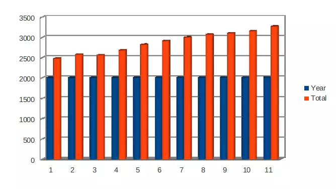
b) Charts of statistical data
Chart of Consumer Price Index from year 2007-2017:

 Chart of Retail Price Index from year 2007-2017:
c) Differences between CPI, CPIH and RPI Indices
|
CPI
|
CPIH
|
RPI
|
|
It can be defined as a weighted average value of purchased goods and services.
|
It refers to new measure of price inflation from ONS (Keller, Â 2015).
|
It is used for revalorisation of taxation or excise duty and uprating the index-linked gilts as well.
|
|
It measures the consumer price inflation which is produced to international standards.
|
It is based on CPI which measures housing costs of goods and services purchased by final consumers.
|
It shows changes in cost of living.
|
|
This method is mostly used by regulatory bodies to determine changes in price of particular products (Melnykov, 2013).
|
This type of technique is used ONS (Office for National Statistics) for publishing a high range of indices which is also called the consumer price index including housing costs. Â
|
It is generally used by business, government and economists for measuring the inflation rate. Â
|
Â
d) Usage of Consumer price Index data for calculating annual inflation
Annual inflation rate can be defined as changes in price of particular products where regulatory bodies use consumer price index method to calculate the same. This would help organisations to decide expansion (Jessop, 2016). As per above national statistical data, consumer value list in the year 2017 has been measured as 1587.6 which is much increased as per previous year 2016 which is approximate 2% as ascended rate of expansion.
e) Importance of determining rate of inflation
Inflation can be defined as increase in price level of certain goods and services over a particular period of time in economy. Whenever price of products are hiked then it directly impacts on purchasing power of people. This would also impact on demand of items also therefore, it affects economical condition of country both in negative and positive manner ( Patéâ€ÂÂCornell, 2012). Government and public organisations measure inflation rate in order to determine expansion rate of economy with cost of living index.
Also Read:Â Developing Global Management Competencies Level 3 GSM london Unit 5
M1 Evaluation of sources other than the NSO with regard to the gender pay gap
It has analysed from National Statistics data that organisations of UK provide employment to male candidates mostly as compared to female. It leads to causes high gender gap as subjected to Consumer Index Price in this nation. For example- As per survey, it has evaluated that under textiles group, the gender pay gap is recorded as 88% that shows it pay less consideration to female working staff then males (Gender pay gap in UK, 2018).
M2 Differences in statistical application in activity 2
In activity 2, for calculating median of given data, O-give curve has used while other  variables like quartiles, standard deviations and interquartile range, frequency distribution has taken. The main difference among both methods is that ogive curve is easy to interpret the result while frequency distribution method requires a tough calculation. But in terms of accuracy, frequency distribution gives more accurate and correct data as compared to graphical representation. Â
D1 Difference between descriptive, exploratory and confirmatory analysis with examples
|
Descriptive
|
Exploratory
|
Confirmatory
|
|
· It aims at exploring the situations of a research in detailed manner.
· It describes  functions and characteristics of data
|
· It focuses on giving insights into and an understand of issues faced by investigators during collection of data.
· It discovers new ideas and thoughts.
|
· It uses traditional methodology like significance, confidence and inference to evaluate evidence of data.
· It covers all basis of gathering, presenting and testing the evidence of data.
|
M3 the use of the statistical methods used in activity 3
In order to manage the inventories and handle stock level properly, it is better to use Economic order quantity analysis, This costing method helps in analysing the optimum quantity of orders, re-orders as well as stock levels. Furthermore, purchasing cost, cost per order and carrying cost is evaluated to analyse inventory policy cost.
D2 Recommendation and judgements made in activity 3
Using economic order quantity, owners of Jenny Jones gets success to manage quality of inventory and complete order of customers on time. Further, it is recommended to its management team to ascertain the reorder level structure for avoiding additional overhead expenses and overcome from shortage of cost as well.
M4 Justification regarding graphical representations used in activity 1 and 2
Bar charts and O-give curve methods of graphical representation are used to represent the data of Activity 1 and Activity 2. O-give helps in evaluating the median and quartiles of data while Bar chart is to represent the CPI and RPI data of Statistical National of year 2007 to 2017.
D3 Use of graphical and tabular representations used in 1 and 2 activities
Both tabular and graphical representation of data is essential to summarise the entire data into single form. Tabular formation is used to represent National Statistics data into quantitative manner which is helpful for analysing data in more appropriate manner. While O-give curve is used to analyse the basic difference among hourly earning by staff member of Manchester and London area.
Activity 2
Hourly pay rates in different regions of UK
a) O-give curve to determine Median
O-give curve can be defined as a statistical tool to measure median of a particular data. It represent data into graphical manner by plotting frequency of data against cumulative distribution functions (Hecke, 2012). In general, O-give curve can be classified into major parts Less-Than and More-than. Under less-than type O-give curve, upper limit of class interval is plotted against corresponding cumulative frequency. While more than type of O-give curve is used lower class limit. The point where both kinds of curves are meet is considered as median of the particular data.
More than O-give curve
|
 Hourly earning in Euro
(Class Interval)
|
No. of Leisure central staff
(f)
|
More than O-give
|
Cumulative frequency
|
|
Below 10
|
4
|
More than 0
|
50
|
|
10 but under 20
|
23
|
More than 10
|
46
|
|
20 but under 30
|
13
|
More than 20
|
23
|
|
30 but under 40
|
7
|
More than 30
|
10
|
|
40 but under 50
|
3
|
More than 40
|
3
|
|
Total
|
50
|
Â
|
Â
|
Less than O-give Curve
|
 Hourly earning in Euro
(Class Interval)
|
No. of Leisure central staff
(f)
|
Less than O-give
|
Cumulative frequency
|
|
Below 10
|
4
|
Less than 10
|
4
|
|
10 but under 20
|
23
|
Less than 20
|
27
|
|
20 but under 30
|
13
|
Less than 30
|
40
|
|
30 but under 40
|
7
|
Less than 40
|
47
|
|
40 but under 50
|
3
|
Less than 50
|
50
|
|
Total
|
50
|
Â
|
Â
|
Â
O-give curve
 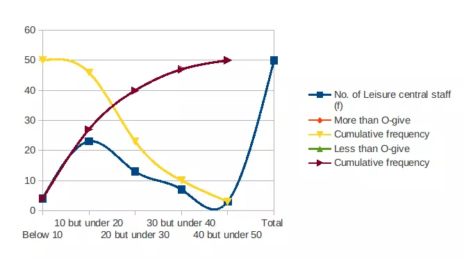
From the above graphical representation, Median obtained is approximate £19.0 for hourly earning for leisure centre staff of London area (Zhou and Luo, 2015). While interquartile range can be obtained as :
Q1 can be defined as first quartile range which is calculated by taking 25% of data. While Q3 is sated as third quartile range that used 75% of total population. Along with this, Inter-quartile range can be defined as a quantum of statistical dispersion it is also known as mid spread  and middle 50%. It is first quartile which is subtracted from third quartile. It is mainly a quota of variability which is based on dividing  of a data set into quartiles. Inter-Quartile is basically a measure where extended values lies.
Q1 = L + (N/4 – cf)/ f X h                      Here l = 10, f = 23, h = 10 and N/4 = ∑F/4 = 12.5, cf = 4
     = 10 + (12.5 – 4)/ 23 x 10
     = 10 + 85/ 23
     = 13.7
Q3 = L + (3N/4 – cf)/ f X h              Here l = 20, f = 13, h = 10 and 3N/4 = ¾ of ∑F = 37.5, cf =27
     = 20 + (37.5 – 27) / 13 x 10
     = 20 + 105/13
     = 28.07
So, Inter-quartile range can be obtained as = Q3 – Q1
                                                                                                                      =  (28.07-13.7)
                                                                      = 14.0 (approx)
b) Mean and standard deviation for hourly earnings of London area
Mean:
It is average of range of quantities or values calculated by adding all data and after then divide it by total of all numbers. End  result is mean or average which is also called arithmetic mean as well. This is most common measure of mid-point in a set of values . It is use to derive central tendency of data in a question (Zyphur and Oswald, 2013). This type of statistical calculation erase accidental errors. This will help to acquire more accurate conclusion. Mean also helps in interpretation of statistical data.
Median:
It is a value that separates higher half from lower half in a given data sample. It is commonly use to measure properties of set of a data. It is very easy to understand and simple to calculate. Median can be use as location parameter in large descriptive statistics. To identify median, an individual arrange observation in a order from small to large value. If odd number is there in observation, then middle value is median (Bedeian, 2014). Whereas if even number is there in observation , then average of two middle value is median.
Standard Deviation:Â
It can be calculated as square root of variance. Standard deviation helps in measuring spread of data about mean value. There are mainly two types of standard deviations which includes population and sample standard deviation. It is a measure which is use to compute amount of given variations in a data value sets. Standard deviations of statistical population, data sets, random variable and probability distribution is square root of their variance (Haimes, 2015). It is mainly use to measure assurance in a statistical conclusion.
You Share Your Assignment Ideas
We write it for you!
Most Affordable Assignment Service
Any Subject, Any Format, Any Deadline
Order Now View Samples
Mean is calculated by taking average of sum of observation as shown below:Â
|
 Hourly earning in Euro
(Class Interval)
|
No. of Leisure central staff
(f)
|
Middle data
Â
(x)
|
Â
Â
(F*x)
|
Middle data
Â
(x2)
|
Â
Â
(F*x2)
Â
|
|
Below 10
|
4
|
5
|
20
|
25
|
100
|
|
10 but under 20
|
23
|
15
|
345
|
225
|
5175
|
|
20 but under 30
|
13
|
25
|
325
|
625
|
4225
|
|
30 but under 40
|
7
|
35
|
245
|
1225
|
8575
|
|
40 but under 50
|
3
|
45
|
135
|
2025
|
6075
|
|
Total
|
50
|
Â
|
1070
|
Â
|
24150
|
Working notes:
Mean = ∑Fx / ∑F
           = 1070/50
           =  21.4
Standard deviation = √ (∑Fx2 / ∑F) - (∑Fx / ∑F)2
                               =  √(24150/50) – (21.4)2
                                                      = √483 – 457.96
                                  = √25.04
                                  = 5. 0 (approx)
Thus, as per above calculation, mean and standard deviation for London area are obtained as £21.4 and £5.0 respectively.
c) Comparison of earning of London and Manchester area
Hourly earning for leisure centre staff in Manchester area:
|
Median
|
£14.00
|
|
Interquartile Range
|
£7.50
|
|
Mean
|
£16.50
|
|
Standard Deviations
|
£7.00
|
Â
Hourly earning for leisure centre staff in London area:
|
Median
|
£19.00
|
|
Interquartile Range
|
£14.00
|
|
Mean
|
£21.40
|
|
Standard Deviations
|
£5.00
|
Â
Therefore, on comparing the above data, it has interpreted that hourly earning for leisure centre staff of London area is more than Manchester area.
More Suggestions:Â
Activity 3
a) Economic Order Quantity (EOQ)
EOQ refers to optimum quantity of goods that can be bought only at one time for minimising the annual total cost  to order holding items in inventory (Barrett and et. al.,  2012). This method is used by organisations in order to minimise cost of inventory as well as can meet needs of customers on time. Â
Economic Order Quantity can be calculated by using below mentioned formula :
EOQ =  √(2 x demand x cost per order) / cost of holding per unit of inventory)
EOQ = √( 2 x D x Co / Ch)
        Where,    D = Demand per year;
                       Co = Cost per order;
                       Ch = Cost of holding per unit of inventory
According to present case, Demand of t-shirt is 2000 and cost per t-shirt is £5; cost of holding=2Â
EOQ = √ (2 x 2000 x 5)/2
         = 100 Units
- b) Re Order tee-shirts
The EOQ method is generally used to measure re-order point through which organisations can control inventories as well as can fulfil demand of customers on time (Andreeva and Kianto, 2012). If any business runs out of its inventory level of stock then it leads to cause shortage in cost. This would also taken as revenue lost as under this condition, company cannot become able to fill an order on time. Therefore, as per present scenario, Ms Jones needs to order tee-shirts in following manner:- Â
Re-order level (ROQ)Â = (Lead time x daily average usage) + safety stock
                                      = (28 x 2)+150
                                      = 206 units
Frequency of Re-order = Demand per year / ROQ
                                        = 2000 / 206
                                        = 9.7 or 10 days
c) Calculation of inventory policy cost
Inventory Policy Cost = Purchase cost + Cost per order + Carrying cost
                                      = 10 + 5 + 2
                                      = £17 Â
The inventory cost is £17 because inventory includes all the cost of maintaining stock.
- d) Current service level to customers
Current Level of service = Demand per week x Availability of t-shirt
                                    =   40 x 95%
                                    =   38 units
- e) Work out the re-order level to achieve desired service level
Re-order level (ROQ) = (Lead time x daily average usage) + safety stock
= (28 x 2) + 150
= 206 units
Activity 4
a) Charts and tables on the basis of office of national statistics produce line
CPI (Consumer Price Index)
Â
|
Year
|
Total
|
|
2007
|
1256.4
|
|
2008
|
1301.8
|
|
2009
|
1330
|
|
2010
|
1373.7
|
|
2011
|
1435.3
|
|
2012
|
1484.9
|
|
2013
|
1513.5
|
|
2014
|
1535.6
|
|
2015
|
1536.3
|
|
2016
|
1546.5
|
|
2017
|
1587.6
|
Retail price index
|
Year
|
Total
|
|
2007
|
2478.6
|
|
2008
|
2577.9
|
|
2009
|
2564.2
|
|
2010
|
2682.7
|
|
2011
|
2822.2
|
|
2012
|
2912.7
|
|
2013
|
2999.5
|
|
2014
|
3072.4
|
|
2015
|
3102.5
|
|
2016
|
3156.6
|
|
2017
|
3269.7
|
Â
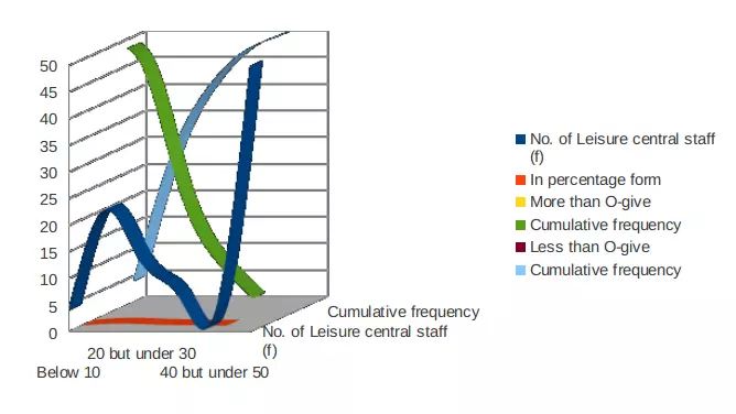
b) An O-give curve of cumulative % of staff versus hourly earning
More than O-give curve of cumulative % staff versus hourly earning
|
 Hourly earning in Euro
(Class Interval)
|
No. of Leisure central staff
(f)
|
In percentage form
|
More than O-give
|
Cumulative frequency
|
|
Below 10
|
4
|
8.00%
|
More than 0
|
50
|
|
10 but under 20
|
23
|
46.00%
|
More than 10
|
46
|
|
20 but under 30
|
13
|
26.00%
|
More than 20
|
23
|
|
30 but under 40
|
7
|
14.00%
|
More than 30
|
10
|
|
40 but under 50
|
3
|
6.00%
|
More than 40
|
3
|
|
Total
|
50
|
Â
|
Â
|
Â
|
Â
Less than O-give curve of cumulative % staff versus hourly earning
|
 Hourly earning in Euro
(Class Interval)
|
No. of Leisure central staff
(f)
|
In percentage form
|
Less than O-give
|
Cumulative frequency
|
|
Below 10
|
4
|
8.00%
|
Less than 10
|
4
|
|
10 but under 20
|
23
|
46.00%
|
Less than 20
|
27
|
|
20 but under 30
|
13
|
26.00%
|
Less than 30
|
40
|
|
30 but under 40
|
7
|
14.00%
|
Less than 40
|
47
|
|
40 but under 50
|
3
|
6.00%
|
Less than 50
|
50
|
|
Total
|
50
|
Â
|
Â
|
Â
|
O-give Curve:
 Â
Â
Conclusion
This mentioned report defines the importance of statistics in collecting, measuring, analysing and interpreting the data. For measuring inflation and deflation period of economy, governmental bodies or organisations can use number of statistical methods. It includes consumer price index, retail price index, central tendencies like mean, median, standard deviations etc. In addition to these methods, tools like economical order quantity can help companies in minimising their inventory cost as well as complete order of customers on time. Â
References
- Andreeva, T. and Kianto, A., 2012. Does knowledge management really matter? Linking knowledge management practices, competitiveness and economic performance. Journal of knowledge management. 16(4). pp.617-636.
- Barrett, K. C and et. al., Â 2012. IBM SPSS for introductory statistics: Use and interpretation. Routledge.
- Bedeian, A. G., 2014. “More than meets the eyeâ€: A guide to interpreting the descriptive statistics and correlation matrices reported in management research. Academy of Management Learning & Education. 13(1).  pp.121-135.
- Haimes, Y. Y., 2015. Risk modeling, assessment, and management. John Wiley & Sons.
- Hecke, T. V., 2012. Power study of anova versus Kruskal-Wallis test. Journal of Statistics and Management Systems. 15(2-3).  pp.241-247.
- Jessop, A., 2016. StatsNotes: Some Statistics for Management Problems. World Scientific Books.
- Keller, G., 2015. Statistics for Management and Economics, Abbreviated. Cengage Learning.
You may also like to read: What Are The Approaches Of Operation Management
Amazing Discount
UPTO50% OFF
Subscribe now for More
Exciting Offers + Freebies


 Super-fast Services