Statistics For Management

Activity 1

a) National Statistical Data

Consumer Price Indices: 

Inflation can be defined as rate of changing price of basic commodities which influence mostly the interest rate on mortgages, saving and more. These rates generally affects state pension level as well as benefits of the same too. CPI refers to measure the inflation rate and purchasing power of national currency (Qiu, Qin and Zhou, 2016). This method expresses current price of basic goods as per difference in price of same year to previous one. It includes bread, meat, milk and other essential household products.

This will indicate effect of inflation on current situation of marketplace. In context with CPIH,  as per National Statistics, it has evaluated that Consumer Price Index which includes housing costs of owners refers to most encompassing measure of inflation. Thus, information provided as per CPI and CPIH helps organisations as well as individuals in estimating the changing price of economy in future also.

Retail Price Index:

RPI is generally used by governmental bodies for several purposes like amount payable on index-linked securities, wage negotiation, inflation rates etc. The data which is not included in CPI such as mortgage interest payments, building insurance, house depreciation and more included in retail price index (Gikhman and Skorokhod, 2015). It also tracks changes in the cost of fixed or basic commodities.

Statistical data in terms of CPI index

Statistical data in terms of RPI Index

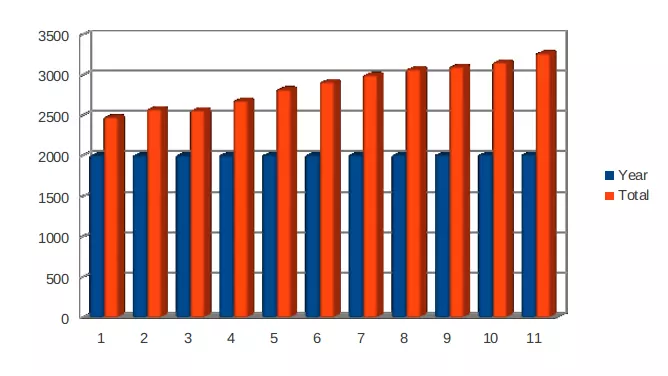
b) Graphical representation of national statistical data

Graphical representation of Consumer Price Index from year 2007-2017:

Graphical representation of Consumer Price Index from year 2007-2017:

c) Differences between CPI, CPIH and RPI Indices

d) Use of collected data form Consumer price Index to determine annual inflation

The consumer price index as per above mentioned national statistical data, Bureau of Labour Statistics reported that it has slightly increased to near about 2% (Lam, 2012). An increase in electricity and gasoline, used cars, trucks and other basic transportation, food items etc. is majorly affect purchasing power of people. Along with this, consumption of some goods like new vehicles, indexes for communication and recreation all, also has also declined slightly from 2016 to 2017.  

e) Significance of calculating inflation rate

Measuring inflation rate is considered as most difficult task for statisticians. For this process, a number of various goods and services which refers to representative of economy will put together in a basket (Keller, 2015). Further, cost of this basket will then compare with past data to analyse the inflation rate. For this purpose, mostly statistician use CPI to measure price changes in goods and services which includes food, gasoline, auto-mobile and more.

Activity 2

Hourly pay rates in different regions of UK

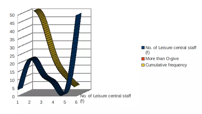
a) O-give curve to determine Median

O-give curve refers to statistical tool which is used for measuring the value of median of a certain data. Under this process, two types of curves are drawn viz. More-than type and Less-than type, where point of inflexion are termed as median of given data. Basically, this kind of curve is drawn on cartesian plan of 2-D data where X-origin represents class-interval and Y-origin shows cumulative frequencies (Jessop, 2016). Concept of both kind of O-give curve can be elaborated by following example:-

More than O-give curve

Less than O-give Curve

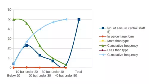
Median determined in terms of More-than and Less-than type O-give curve:

Therefore, the point where both kinds of O-give curve that are less-than and more-than is considered as Median. From this process, median for hourly earning for leisure centre staff of London area is calculated as near about £19.0.

Quartile:

A quartile is a statistical term which helps to define or explain a division of observations into four equal intervals based upon values of data and how they are used to compare entire set of observations (Walters, 2016).

• First quartile: It is denoted by Q1 and is termed as median of lower half of any given data set. This can further be said that 25 % numbers lie below Q1 and 75% lie above it.
• Third quartile:It  is symbolically represented by Q3 and is known to be median of upper half of any given data set. So, this can further be said that 75% numbers fall under Q3 and 25% lie above it.

Interquartile:

Inter quartile or inter quartile range is a statistical measure of variability. It is based on dividing any given data set into quartiles.

Now Quartiles can be calculated as per:-

Therefore, First Quartile of deviation can be calculated as per:-

 Here lower limit (l) = 10, frequency (f)

= 23, Class interval (h)

= 10 and Total frequency (N/4)                        

 = ∑F/4 = 12.5, cf = 4

Q₁ = L + (N/4 – cf)/ f x h                   

     = 10 + (12.5 – 4)/ 23 x 10

     = 10 + 85/ 23

     = 13.7

While, Third Quartile of deviation can be calculated as per:-

   Here l = 20, f = 13, h = 10 and 3N/4 = ¾ of ∑F = 37.5, cf =27

Q₃ = L + (3N/4 – cf)/ f x h           

     = 20 + (37.5 – 27) / 13 x 10

     = 20 + 105/13

     = 28.07

Therefore, Inter-quartile range can be calculated by measuring the difference among first and third quartiles, as shown below:-

   IQR =   Q_{3 –} Q₁

                   =  (28.07-13.7)

            = 14.0 (approx)

b) The mean and standard deviation for hourly earnings of London area

Central tendency can be defined as process to show entire data into single manner. This method is given by Professor Bowley which has given various types of techniques to calculate and analyse large information into simpler form (Hecke, 2012). It includes mean, median, mode, quartiles, standard deviations and more. Concept of some of these methods can be explained in following manner:-

Mean:

It can be defined as an average of a particular data which can be measured by dividing sum of observation to total numbers. It is also known as arithmetic mean of data which covers entire observations. Therefore, in present context, this methodology helps in calculating average of hourly earning  for leisure centre staff in London area.

Median:

It refers to middle data or second quartile of central tendency which denotes the midpoint of a frequency distribution (Haimes, 2015). It is calculated by various methods like O-give curve, frequency distribution method and more.

Standard Deviation: 

It can be defined as a measure of central tendency which is used to quantify the amount of dispersions or variations of a set of values.  

Mean is calculated by taking average of sum of observation as shown below: 

Calculation

Mean = ∑Fx / ∑F

           = 1070/50

           =  21.4

Standard deviation= √ (∑Fx² / ∑F) - (∑Fx / ∑F)²

            =  √(24150/50) – (21.4)²

            = √483 – 457.96

           = √25.04

           = 5. 0 (approx)

Thus, as per above calculation, mean and standard deviation for London area are obtained as £21.4 and £5.0 respectively.

c) Comparison of earning of London and Manchester area

Hourly earning for leisure centre staff in Manchester area and London area

Therefore, on comparison of hourly earning of both area of Manchester and London, it has analysed that

Activity 3

a) Economic Order Quantity (EOQ)

EOQ is the order quantity that determine the total cost and ordering cost. It is considered as one of the most classical production planning methods which was developed by Ford W.Harris  in 1913. In depth analysis, EOQ method can be altered to find out  different production standard or can be stated as fundamental techniques with large supply series to calculate variable cost (Bedeian, 2014).

Economic Order Quantity can be calculated by using below mentioned formula :

EOQ = √( 2 x D x Co / Ch)

 Where,    D = Demand per year;

 Co = Cost per order;

Ch = Cost of holding per unit of inventory

As per present case study,

Demand of t-shirt = 2000;

cost per t-shirt is £5 and

cost of holding=2 

Therefore, EOQ = square root of (2 x 2000 x 5)/2

 = 100 Units

1. b) Re Order tee-shirts

 It is essential for companies to have a knowledge about dimension of crude and completed stock which helps in increasing effectiveness of production process (Barrett and et. al.,  2012). In case of loss of control on inventory level of stock, an organisation can face problems like shortage in cost. Therefore, under such condition, firm will also not in state to cover revenue as well or meet demand of customers on time.

In context with present case, Ms Jones are required to re-order following number of tee-shirts as shown in below calculation:-  

Re-order level (ROQ) = (Lead time x daily average usage) + safety stock

 = (28 x 2)+150

= 206 units

Frequency of Re-order = Demand per year / ROQ

= 2000 / 206

= 9.7 or 10 days

c) Calculation of inventory policy cost

It is essential for organisations or individuals to calculate inventory policy cost so that expenses can be reduced and manage stock also (Andreeva and Kianto, 2012).

Inventory Policy Cost = Purchase cost + Cost per order + Carrying cost

= 10 + 5 + 2

 = £17  

As inventory covers all kinds of expenses and cost of managing stock therefore, it is obtained as £17.

1. d) Current service level to customers

Current Level of service = Demand per week x Availability of t-shirt

=   95% of 40

=   38 units

1. e) Work out the re-order level to achieve desired service level

Re-order level (ROQ) = (Average usage x Lead time) + additional stock

= (28 x 2) + 150

= 206 units

Activity 4

a) Charts and tables on the basis of office of national statistics produce line

CPI (Consumer Price Index)

Retail price index

b) An O-give curve of cumulative % of staff versus hourly earning

More than O-give curve of cumulative % staff versus hourly earning

Conclusion

From this assignment it has analysed that to analyse any data in appropriate manner, mostly organisations use statistical concepts. It provides various methods like central tendencies,  deviations, dispersion and more which helps in analysing data in simple manner. An effective knowledge of statistics as well as ability for applying such applications can help in resolving various problems.  

References

• Andreeva, T. and Kianto, A., 2012. Does knowledge management really matter? Linking knowledge management practices, competitiveness and economic performance. Journal of knowledge management. 16(4). pp.617-636.
• Barrett, K. C and et. al.,  2012. IBM SPSS for introductory statistics: Use and interpretation. Routledge.
• Bedeian, A. G., 2014. “More than meets the eye”: A guide to interpreting the descriptive statistics and correlation matrices reported in management research. Academy of Management Learning & Education. 13(1).  pp.121-135.
• Haimes, Y. Y., 2015. Risk modeling, assessment, and management. John Wiley & Sons.
• Hecke, T. V., 2012. Power study of anova versus Kruskal-Wallis test. Journal of Statistics and Management Systems. 15(2-3).  pp.241-247.
• Jessop, A., 2016. StatsNotes: Some Statistics for Management Problems. World Scientific Books.

UPTO50%

Avail The Benefit Today!

To View this & another 50000+ free

Enter Email

Submit